Using ML and AI for stock price prediction
Posted on 2025-02-20 16:13:37
Welcome back to yet another journey into AI (still highly caffeinated—Yorkshire Tea is the best brand of tea). If you haven't read my first AI article, I'd recommend doing so here. Otherwise, the TL;DR is that I'm brand new to the whole AI development thing, and I'm trying to publish a research paper by the end of the year. I have recently learned how PyTorch, NumPy, and some of the AI maths work, so I'm going to skip the basics that I went over in the last article. By the end of the blog, I had a working OCR model. In this article, we’re hopefully going to have a working long short-term memory (LSTM) model to predict stocks.
So, what is an LSTM model?
An LSTM is a type of recurrent neural network (RNN). This means that before I can explain what an LSTM is, I'm going to have to take a few steps back and explain what an RNN model is. An RNN is a type of AI model designed to be used with sequential data (data that is organised in a sequence, where the order is important), such as sentences, sensor measurements, gene sequences, and, you guessed it, stock prices. RNNs are one of the few models that have a kind of memory. The memory in an RNN is called a hidden state, and this is fed through a loop.
This might be a bit hard to understand, so let's put this in an example. Let's say we are reading a sentence.
The first word gets passed into the RNN model, and the model generates a hidden state. (To make life simple, just think of a hidden state as a summary of what the model has been exposed to so far.)
Next, the following word is given to the RNN model, along with the hidden state that was generated by the previous word. An updated/new hidden state is created.
The model then continues to loop through the sentence, passing on the previous hidden state.
If you are interested, this process can be shown as a
Where:
- ( x_t ) = current input (e.g., a word at time ( t ))
- ( h_{t-1} ) = previous hidden state (memory from the last step)
- ( W, U, b ) = learned parameters (weights and biases)
- ( f ) = activation function (usually tanh or ReLU)
If you don't understand the maths, that's not important. I've kind of left it in for those who are interested. I'm happy to go through it over on Discord, but don't worry about it too much.
The downside of RNN models is that they can sometimes forget things. This is called the "vanishing gradient problem". As the model takes in more data, the weighting of earlier data decreases. It can eventually decrease to the point that it's no longer significant. This is because the gradients shrink exponentially during backward propagation.
One of the main benefits of an LSTM is that it fixes the vanishing gradient problem. LSTMs use a structure called a memory cell, which allows them to selectively remember or forget information over long periods. The memory cells have three gates.
- Forget Gate: Decides which information to discard from the cell state.
This gate decides which parts of the previous cell state should be
kept or discarded. It takes the previous hidden state and the current
input and outputs a number between 0 and 1 for each value in the cell
state. If the number is closer to one, it is kept. If it's closer to
zero, it's forgotten.
- Input Gate: Determines what new information should be added to the cell state.
- Output Gate: Controls what information from the cell state should be used as output.
Now, if you are feeling fancy, you can chain LSTMs together. You do this by taking the state of the previous cell as well as the output and feeding that into the new cell with an input. This cell then processes its own outputs, and so on. This process enables LSTMs to learn dependencies over long sequences while reducing the vanishing gradient problem. I think this is all the information that's needed for us to start coding.
The first new thing is making a DataFrame. LSTMs require sequential data, so we need to make a table where we shift back the closing prices. I have decided to do this a week at a time.
def prepare_dataframe_for_lstm(df, n_steps):
    df = dc(df)
    df.set_index('Date', inplace=True)
    for i in range(1, n_steps + 1):
        df[f'Close(t-{i})'] = df['Close'].shift(i)
    df.dropna(inplace=True)
    return df
This creates an output that looks like this. (This is not the full output, but trying to format code blocks is hard. You get the idea.)
               Close  Close(t-1)  Close(t-2)  Close(t-3)  Close(t-4)
Date
1997-05-27  0.079167    0.075000    0.069792    0.071354    0.081771
1997-05-28  0.076563    0.079167    0.075000    0.069792    0.071354
1997-05-29  0.075260    0.076563    0.079167    0.075000    0.069792
1997-05-30  0.075000    0.075260    0.076563    0.079167    0.075000
1997-06-02  0.075521    0.075000    0.075260    0.076563    0.079167
1997-06-03  0.073958    0.075521    0.075000    0.075260    0.076563
1997-06-04  0.070833    0.073958    0.075521    0.075000    0.075260
1997-06-05  0.077083    0.070833    0.073958    0.075521    0.075000
1997-06-06  0.082813    0.077083    0.070833    0.073958    0.075521
1997-06-09  0.084375    0.082813    0.077083    0.070833    0.073958
After this, we need to normalise the data. By normalising the data, we make the minimum value -1 and the maximum value 1. This will speed up convergence. Stock prices can end up being massive numbers, which leads to large gradients, either slowing down convergence or causing unstable training (large or rapid changes in gradients, or the loss function fluctuating instead of decreasing).
The next few steps are boring, so we will just brush over them: converting everything to NumPy, splitting the data into X and Y, reshaping the data, and then converting it to tensors. Finally, we split the data into testing and training sets. The first 95% of the data will be used for training, and the last 5% will be used for testing.
Now for the fun part—creating the model. Making an LSTM is surprisingly simple with PyTorch. Our class takes in four attributes: input size, hidden size, number of layers, and output size. We are using an input size of 1, so we are processing one row of the table at a time; a hidden size of 4, meaning we are using four nodes in every LSTM; and one layer, meaning we are using a single LSTM model. This is due to it being a simple problem—chaining multiple LSTMs together can lead to overfitting. This is also the reason for using so few nodes. ("Overfitting means creating a model that matches (memorises) the training set so closely that the model fails to make correct predictions on new data" — Google Developer Crash Course). Finally, there is only one output, as the only data we want to take from the model is the future price of the stock.
class LSTM(nn.Module):
    def __init__(self, input_size, hidden_size, num_layers, output_size):
        super(LSTM, self).__init__()
        self.hidden_size = hidden_size
        self.num_layers = num_layers
        self.lstm = nn.LSTM(input_size, hidden_size, num_layers, batch_first=True)
        self.fc = nn.Linear(hidden_size, output_size)

    def forward(self, x):
        batch_szie = x.size(0)
        h0 = torch.zeros(self.num_layers, batch_szie, self.hidden_size).to(device)
        c0 = torch.zeros(self.num_layers, batch_szie, self.hidden_size).to(device)
        out, _ = self.lstm(x, (h0, c0))
        out = self.fc(out[:, -1, :])
        return out

model = LSTM(1,4,1,1).to(device)
Next is the forward function. The first thing is initialising the memory (hidden and state cells) with zeros. For every batch of the training loop, there is no previous data, so if we did not create a tensor of zeros, the computer would use random values from the system's memory. This would lead to a bias in the data.
The next step is passing in the current batch and memory into the LSTM. This step returns two things: a tensor with the output values and the memory in the final state. We don’t need the values of the memory, so we cast it into the void (assign it to a _ variable, which is a convention in Python to indicate unused or unnecessary data). We then output and extract the last time step from the tensor. Finally, the extracted data is passed into a fully connected layer, leading to our single-value stock price output.
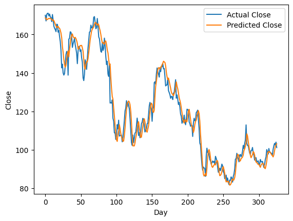
This model goes through several training loops (also explained in the last article), and then we compare our predicted data to the real data. The model seems fairly accurate.
Now for the fun part. Getting rich quickly. I have this rather crude trading strategy code.
initial_cash = 1000
cash = initial_cash
shares = 0
portfolio_value = []

buy_threshold = 1.01  # Buy if the predicted price is 1% higher than current
sell_threshold = 0.99  # Sell if 1% lower
position_size = 0.1  # Allocate 10% of cash per trade

for i in range(1, len(new_y_test)):
    current_price = new_y_test[i]
    predicted_price = test_predictions[i]

    if predicted_price > current_price * buy_threshold and cash >= current_price:
        shares_to_buy = (cash * position_size) // current_price
        shares += shares_to_buy
        cash -= shares_to_buy * current_price
    elif predicted_price < current_price * sell_threshold and shares > 0:
        cash += shares * current_price
        shares = 0

    portfolio_value.append(cash + shares * current_price)
Now, could this code be better? Yes, but the goal of this project was the AI aspect. In short, we look at the current value and our predicted future value. If it’s ≥1% higher, we buy stock; if the future value is ≥1% lower, we sell the stock. Now for the bit of information everyone wants: how much PROFIT did this make?
By giving it a (fake) 1000 USD and letting it run between the years of 2021-12-08 and 2023-04-05 (with a speed-up in simulation time), a grand total profit of 22.99 USD was made.
Now, is this a success?
Kinda. I have successfully created a working LSTM model that generates profit. However, if you had put the same 1000 USD into a 4.4% ISA, you would have made 59 USD of profit. But hey, that's less fun.
If you enjoyed the blog, feel free to join the Discord or Reddit to get updates and discuss the articles. Or follow the RSS feed.